<##CLIENT##> Family Trust |
27 February 2017 |
We have recommended that you invest $270,000 in the Wingate Global Equity Fund. I have prepared this section to help explain the reasons behind this decision, and to help you understand how the strategy works.
About the strategy
The Wingate Global Equity Fund is a long-only, value-oriented strategy which incorporates derivatives to both enhance income and support the purchase of sale and purchase of securities at prices they believe provide investors with a reasonable return on their equity.
The strategy contains a number of unique features. For example, while the strategy has significant derivatives exposure, the portfolio does not use leverage. This is because the Fund only writes options on assets it either already owns (in the case of Call options), or can afford to own via a special cash reserve (in the case of Put options).
As the Fund only writes options (and does not buy them), they earn a premium for the options sold. The structure of options essentially means the Fund is entering into a contract with the purchaser whereby Wingate will either sell their shares a predetermined price (in the case of Calls), or buy at a predetermined price (in the case of Puts). This means that Wingate’s potential profit from an equity holding is limited by the price at which the call is set (plus dividends and option premium income, of course). This means that options will only be exercised by the purchaser if the share price rises above the option Strike price. Their Put option exposure, on the other hand, is an agreement that Wingate will buy stock at a specified price, meaning that the option will only be exercised if the share price falls below a certain price; in this case Wingate will have to buy the shares at the strike price, even if the actual share price has fallen much further.
Importantly, while the strategy is long-only equity (meaning they cannot take “bets” on stock prices falling), the strategy entails holding sometimes-large levels of cash. Cash holdings comprise the portion of the portfolio set aside to cover Put contracts, if exercised, plus up to 20% which may be held at the manager’s discretion. This flexibility adds another dimension to the strategy as it allows the manager to adjust the portfolio’s risk exposure. For example in the current market, where many equity assets appear quite expensive, the manager could sell Call options closer to the current price of shares in their portfolio (which would yield a higher option premium), while selling Put options at lower prices (which would yield a lower option premium). This in turn allows the portfolio to become more and more conservative the higher that share prices go above what analysts consider to be “fair value”, while still generating a return far above what is possible from cash.
An example:
Perhaps the best way to explain their strategy is through an example.
Let’s say there are two companies. Both are listed on the stock exchange and both of which the investment manager really likes. Company A is a technology company, which Wingate has valued at $110. Company B is a technology company that Wingate has valued at $95. As it happens, both companies are currently trading on the stock exchange at $100 and both pay quarterly dividends of $1 per share.
The way Wingate’s strategy works (at a broad conceptual level) Wingate would purchase Company A for $100, however they have already decided that $110 is a fair value for the company, so they agree that if the share price hits $115 in the next few weeks they will sell their shares. Wingate would also really like to add Company B to their portfolio, however at $100 it is well above their fair value estimate of $95. Their analysts decide that if the share price dropped to $90 the company would be a bargain, so they would buy it.
To look at how it works from a practical investment perspective, let’s say they would like to have 1,000 shares in each company.
Company A
As the current share price is below their estimate of fair value, they buy 1,000 shares at $100 ($100,000). They also confirm that they would be willing to sell at a price of $115 by selling 1,000 call options at a strike price of $115. The options last for the next three months; if the share price does not reach $115 the call option will expire worthless. In selling these call options they receive $0.95 per share, or $950. So long as they own the shares they also receive dividends. The maximum profit that can be earned from this trade over the next three months is $15,000 ($15 per share) from share price appreciation, $1,000 in dividends, plus $950 from option premium. So if they are forced to sell (i.e., the Call option is exercised), they still walk away with a return of around $16,950 (16.95%). Not bad for three months.
Company B
With the analysts deciding that buying Company B’s shares for $90 would be a bargain, Wingate decides to sell 1,000 put options at a strike price of $90. For this, they receive $0.80 per share, or $800. To ensure they have money available to buy these shares, they also set aside a cash position to ensure they can fulfill their obligations to the Put contracts if exercised. To do this they transfer $90,000 (1,000 x $90) to cash. If Company B’s share price does not fall below $90 per share, the put option will not be exercised, and the return on investment from the trade will be equivalent to the cash return on the money put aside ($90k x 2%/4 = $450) plus option premium of $800; in total $1,250 or 1.39%. That’s an equivalent return of around 5.7% per annum for what is essentially a cash position. If Company B’s share price falls below $90 they will take ownership of the shares at a price of $90, even if the price falls much lower than this.
As a result of this strategy there are three components to their portfolio:
- Equity: this is the proportion of their portfolio invested in shares (eg. $100,000 in Company A)
- Cash to cover Puts: this is also cash, however has been reserved to pay for assets that they have offered to buy at a lower price than is currently available in the market (eg, Company B; therefore $90,000 is set aside in cash to cover this position)
- Cash (unencumbered): this is simply the cash within their portfolio they have available to direct to other purposes. For example, the total amount available for investment, after the trades mentioned above, we would have $10,000 ($200,000 - $100,000 - $90,000 = $10,000) allocated to this account (plus about $1,750 from option premiums)
Some of the unique characteristics of this strategy
Dynamic in nature
This structure of the strategy makes it dynamic in nature. Pre-determined valuation thresholds (the points at which options are written) means that the proportion in invested in shares reduces as equity prices rise, and increases when prices fall. Consider how this interacts with our broader portfolio; when equity prices fall (reducing our market exposure) this strategy steps in to make up the difference. Similarly, when prices peak higher this strategy locks in profits.
Benefits from volatility
At first it might seem counterintuitive, but with this strategy volatility is a good thing. For one, it provides more opportunities for share prices to peak higher and dip lower, allowing us to exercise our options. The increased probability of claim, represented as a function of volatility is one of the primary determinants of option price (Black-Scholes Model). This means that the premium we can be paid for selling options, regardless of whether they are call or put options, is higher; for example, instead of being paid $0.80 per option we might get $1.20. The downside is, of course, that we trade away our right to benefit from the more extreme highs and lows of markets, however when incorporated alongside traditional equity portfolios and long/short strategies we see that the penalty is actually very small.
A note on option pricing
The mathematics of option pricing can get a little bit confusing, and involves understanding things like Brownian Motion (a concept borrowed from physics), implied volatility and convexity of time-value. Fortunately computers do most option pricing these days, so we can get away with just concentrating on the broad concepts. Perhaps the easiest way of thinking about it is to understand how options look from the option buyer’s perspective. Most options traders are large, professional investors who use options to manage risk, thus their motivating factor is usually not profits but risk management (a bit like how insurance companies pay reinsurers to absorb some of their risk). From a pricing point of view, options are priced so that the cost is roughly equivalent to the risk-free rate of borrowing plus the probability of claim over the time between now and expiry of the option; the probability of claim is incorporated into a measure known as the Delta. Of course the formal option pricing formula is much more exact, however as previously stated you don’t need to know it to understand the basics concepts behind option pricing. Because investors can’t (in the real world) borrow at the risk free rate, and because transactions usually involve administration costs and the employment of people, the person buying the option will nearly always be entering into a contract in which they expect to make a net loss, roughly equivalent to the interest margin they pay on top of the official risk-free rate. Once this concept is understood it is fairly easy to see that the person writing the option is being paid roughly the equivalent of the risk-free rate of return on their notional exposure of assets underlying the option (so in this case the shares the options are written over), multiplied by a measure that reflects the probability of claim between now and expiry of the option (the Delta), less the risk-free rate multiplied by the option price. As a result, there is a positive correlation between both volatility and option prices and interest rates and option prices. This means that if volatility increases (as we would expect in times of market crisis), so too will the price of options, thereby increasing the amount of income earned from the option-writing components of this strategy (both on Puts and Calls).
Probability illusions
Another point that isn't reflected in options-pricing models is that movement in the price of the underlying shares means that probabilities do not remain constant. Another example. Let's say that you owned a share that you feel is worth around $100, but it's price is very volatile. Around one in every three years it hits a price either below $70 or above $130 (i.e., 1 standard deviation = ~30%). If the underlying price is $100 we might be able to neatly calculate an options price with volatility of 30%. However what happens if the price dips to $80, or spikes to $120? Should we value options based on an underlying price of $80 or $120? The answer is yes. Should we still assume volatility of 30%? The answer again is yes. However, if we do, then a 1-standard deviation event for our option price would be adding-or-subtracting 30% volatility from an inflated or depressed price. Consider this: a price of $120 would be expected to occur around once every four years. From a price of $120, a 30% spike would bring a price of $156 At 30% volatility, from a price of $100 we have a roughly 15% chance (one in 6.7 year event) of ending the year at a price above $130, but only a roughly 3% chance (one in 33 years) of price above $154. In applying this to an option-writing strategy, we see that the timeframe covered by options is very important. Had we written a call option over our shares when they were trading at $100, then an option with a strike price of $130 (at 1-standard deviation from $100) would be worth significantly more than when we sold it. But if the option expires, we then have the opportunity to write another option. If the motive behind our option writing is to generate income and "lock in" what we see as a fair sale price, then we might decide to write a new option at strike $130, which is a price only $10 (8.3%) above the current price, and only about 1/3 standard deviation above the current price. This in turn would yield a much more valuable option premium, even if (in the analyst's opinion of asset fair value) there has been no change.
Currency
Wingate offer both a hedged and unhedged version. On our assessment of the current market and economic environment we prefer the unhedged version. Our current exchange rate is one Australian dollar for USD$0.78. We expect this to weaken in the years ahead. Our recommendation to leave currency exposure unhedged is based on a number of factors, in particular:
(1) Interest rate differentials: The market is currently forecasting four rate-rises from the United States between now and the end of 2018; compared against Australia’s monetary position, which points toward further easing if it can be accomplished without further exacerbating household debt levels, we see that for the $AUD to find additional strength we would need to see our country risk premium reduce significantly, or a spike in growth and inflation. This is not to say this isn’t possible, however it seems incredibly unlikely given how much of our growth is dependent on China’s growth ambitions and the threat of a more protectionist United States (BAT etc).
(2) Australian residential property prices: When we talk of interest rate differentials, and the risk premiums implied in exchange rates, we tend to concentrate our discussion on broad economic growth and inflation trends (covered interest rate parity, or IRP for short). One of the problems with IRP models is that it provides a poor measure of tail risk; that is, the risk that unexpected but significant events can have on currency values. Australia’s residential property prices present one of these risks. Risk-adjusted valuations are massively out of balance (overpriced in real terms by 30% - 40%) and with slowing wages growth, rising dependency rations, rising household size and continued high levels of household debt all suggest that it is a matter of when, and not if, we see prices correct. The flow on effects will likely include: contraction in the construction sector, increase in defaults, reduction in credit growth, lower consumer spending (“wealth effect”) and a high likelihood of recession. All of which point toward a more accommodative monetary and fiscal response coupled with a period of lower economic growth.
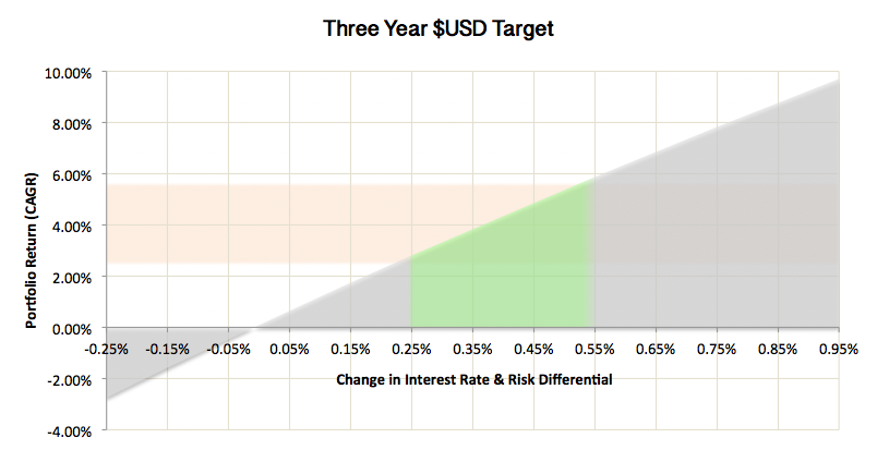
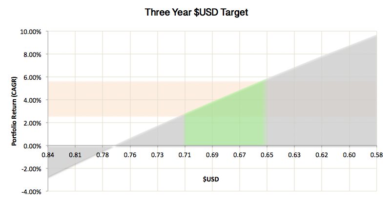
While we are not game to forecast where the $AUD will be in one, six or twelve months (and it doesn’t really matter), we can make some longer term predictions based on different economic growth scenarios. Below present our three-year Australian-United States exchange rate forecasts. Assumed hedging costs at 0.1% p.a. (total returns in brackets):
Our outlook for the next three years is for the interest rate and risk differential to widen by between 0.25% and 0.55%, suggesting that the Australian dollar will weaken to less than USD$0.71. Over a three-year period, this equates to a difference in annual return of between 2.80% and 5.86% p.a.
(1) Interest rate differentials: The market is currently forecasting four rate-rises from the United States between now and the end of 2018; compared against Australia’s monetary position, which points toward further easing if it can be accomplished without further exacerbating household debt levels, we see that for the $AUD to find additional strength we would need to see our country risk premium reduce significantly, or a spike in growth and inflation. This is not to say this isn’t possible, however it seems incredibly unlikely given how much of our growth is dependent on China’s growth ambitions and the threat of a more protectionist United States (BAT etc).
(2) Australian residential property prices: When we talk of interest rate differentials, and the risk premiums implied in exchange rates, we tend to concentrate our discussion on broad economic growth and inflation trends (covered interest rate parity, or IRP for short). One of the problems with IRP models is that it provides a poor measure of tail risk; that is, the risk that unexpected but significant events can have on currency values. Australia’s residential property prices present one of these risks. Risk-adjusted valuations are massively out of balance (overpriced in real terms by 30% - 40%) and with slowing wages growth, rising dependency rations, rising household size and continued high levels of household debt all suggest that it is a matter of when, and not if, we see prices correct. The flow on effects will likely include: contraction in the construction sector, increase in defaults, reduction in credit growth, lower consumer spending (“wealth effect”) and a high likelihood of recession. All of which point toward a more accommodative monetary and fiscal response coupled with a period of lower economic growth.
While we are not game to forecast where the $AUD will be in one, six or twelve months (and it doesn’t really matter), we can make some longer term predictions based on different economic growth scenarios. Below present our three-year Australian-United States exchange rate forecasts. Assumed hedging costs at 0.1% p.a. (total returns in brackets):
- Australian economic growth lifts 1.0%, US trend growth: USD$0.84 (-8.0%)
- Australian trend growth, US trend growth: USD$0.81 (-4.7%)
- Interest rate differential widens 0.25%: USD$0.71 (+8.6%)
- Interest rate & risk differential widens 0.55%: USD$0.65 (+18.6%)
- Interest rate & risk differential widens 0.85% USD$0.60 (+28.6%)
Our outlook for the next three years is for the interest rate and risk differential to widen by between 0.25% and 0.55%, suggesting that the Australian dollar will weaken to less than USD$0.71. Over a three-year period, this equates to a difference in annual return of between 2.80% and 5.86% p.a.
|
|
Currency exposure also helps balance returns from your domestic exposure to shares and property (including your family home) as deterioration in local economic conditions will be partially offset by enhanced returns from your global equity portfolio. This is essentially an “each way bet”: if Australian economic conditions strengthen considerably and outperform the United States, we will feel the uplift in our local assets (Australian shares, your home value etc.), while our currency exposure will record a loss. On the other hand, if economic conditions do deteriorate your losses on domestic assets will be partially offset by currency gains, which then enable us to use this opportunity to bring currency profits back to Australia and invest in assets at depressed prices.
One final aspect of this strategy’s currency exposure that is worth understanding what happens if equity prices fall on a global scale. Were this to happen we would expect a shift toward traditional safe-haven asset, such as the USD and CHF. As Put options are all cash-backed we would not expect to see any currency loss on the option exercise, potentially allowing us to offset or mitigate losses through a weakening $AUD. However in the case where equity prices rise, the exercise of Call options could potentially force us to realise a loss on our currency exposure while making it more expensive to re-establish equity exposure. The two scenarios in which they may happen are either a sudden and unwarranted spike in equity markets (in which case we would be happy to sit on the sidelines), or if the Fund’s analysts make poor investment decisions.
Of course the question must be asked that if we do expect interest rate and risk differentials to widen, why wouldn’t we simply divest from Australia and invest instead into hedged global equities? While this is a fair point (and is already partly reflected in our asset allocation targets), we do acknowledge that despite Australia’s headwinds (of which there are many), we are still able to extract a return premium on Australian equities. The premium is not what it used to be, but is still hovering around the 3.5% - 5% range, which from a global perspective is pretty good.
Performance & Risk
Historical Returns
From a simple benchmark-relative perspective, the Wingate Global Equity Fund appears to be chronic underperformer. The fund uses the MSCI World (ex Aust) as the Fund’s benchmark, though I would argue that this does not adequately reflect the net risk of the fund (currently holds only 47% in shares and 34% of Put option cover). Over the 12 months to 31 January 2017 the strategy generated a return of 5.45%, underperforming the benchmark by 3.4% per annum. Over five years the Fund underperformed by 4.4% per annum (13.33% vs. 17.74%), delivering a compound return of 87% versus 126% for the benchmark.
As discussed previously, the risk profile of this strategy is substantially different to a normal long-only equity Fund. With the Fund currently adopting a relative conservative equity exposure we should expect to underperform if markets rise by more than a few percent above cash, and outperform if equity prices remain flat of decline. Furthermore, we should expect some spikes in returns (more cash flow from option premiums) as volatility increases.
In comparing performance I would suggest a better measure of risk would be to compare returns against a benchmark that reflects against the underlying market risk. I discussed this with Wingate’s CEO recently and he has kindly prepared the following chart which illustrates the portfolio’s return compared to the expected returns from their underlying market exposure (this is simply the market returns multiplied by the amount their exposure to the market, represented as Delta):
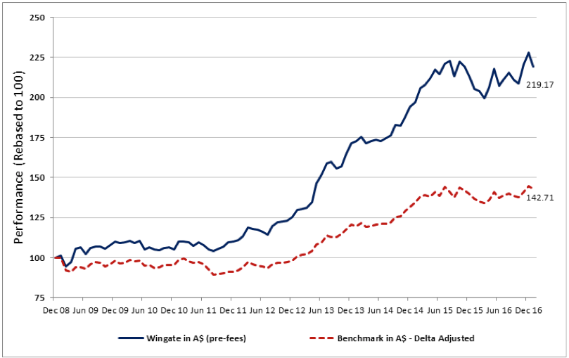
What this illustrates is that Wingate’s analysts have shown skill in their stock selection and option-writing strategies, though it should be said that these results are not surprising over a normal market cycle as their delta-adjusted exposure doesn’t show how many times they have been forced to sell early. The somewhat more volatile performance of the Fund can, in part, be attributed to the fall in market volatility that has made it more difficult to earn a decent income from option premium.
As always, we hold no loyalty to Fund managers. The inclusion of this strategy in your portfolio will serve our objectives of enhancing returns (on a cash relative basis) while dynamically increasing our exposure to assets should markets weaken. In the event of significantly softer asset prices we will most likely reallocate this capital toward more less constrained strategies (i.e., without Calls that limit upside).
As always, we hold no loyalty to Fund managers. The inclusion of this strategy in your portfolio will serve our objectives of enhancing returns (on a cash relative basis) while dynamically increasing our exposure to assets should markets weaken. In the event of significantly softer asset prices we will most likely reallocate this capital toward more less constrained strategies (i.e., without Calls that limit upside).
Investment Return Targets
Based on the Fund’s current asset allocation, our medium-term return forecast for the Fund includes option premium income of 4.3%, dividend income of 1.4% and ex-fees capital growth of 0.4% (total 6.1%). We further anticipate currency to add approximately 6% to returns over the next three years, bringing our total mid-term return target to 7.8% p.a. (+25.4% over next three years, comprising 19.4% investment return, 6% currency). Underlying market exposure is currently 45%; we anticipate this falling to under 20% for market peaks over 20% and rising to 75% for market falls in excess of 20%. With this beta adjustment (dynamic exposure to market risk) on a relative basis we expect this strategy to underperform at times where markets returns exceed 11% p.a.
Fund Risk Targets
The fund currently holds equity exposure of around 47%, with Put cover of 34%, plus 20% unencumbered cash. As the Fund is opportunistic in nature, the level of underlying risk will vary, however the value-focused nature of their valuation process means that even in a 100% equity portfolio total risk will be below-market. In rough terms, we would expect a mid-term risk (volatility) target equivalent to around 60% of market, or somewhere around 8% - 9% per annum, but with much shorter “tails” (in other words, the distribution of returns are more clustered in the middle). Moreover, on analysis of the period 9 July 2012 to 9 February 2017 (1,678 days) we find that the Fund’s return shows a very low 0.35 correlation with the market. As we are not investing in this Fund as a single, standalone asset, we must consider risk and return in a total portfolio context. In this light, we find that real volatility attributable to this strategy is most likely closer to 4%. Therefore, inclusion of this portfolio is expected to generate a return of ~7.8% per annum for risk of ~4% per annum. At an assumed risk-free rate of 2% this suggests an Information Ratio (IR) of approximately 1.45, well above our target IR of 1.00 and above our nominal return objective, while offering an adjusted risk target below our IPS risk target.
Sortino Ratio
To further check that the Fund provides an adequate reward for risk we also assess the portfolio against what is known as a Sortino Ratio. This ratio illustrates what level of downside risk we are exposed to for each unit of return we achieve above our target.
We apply a somewhat modified version of Sortino, using a 60-trading day (approximately 3 month) moving average to capture our return targets. This approach tends to exaggerate the effects of market downturns, which I believe helps to better illustrate the risk of holding an asset from an individual investor’s perspective (in effect we are looking how much capital we are risking over a three-month period).
The results follow results from the past 12 months. As you can see, the Portfolio (which in this case only refers to your equity-linked assets) plus Cromwell), with a Sortino Ratio of 0.87 against our target return, suggests that at a 5.66% risk target specified in your Investment Policy Statement would have allowed us to add 4.92% of return above and beyond your IPS return target, when in reality your portfolio over the past 12 months actually achieved a relative outperformance of 13.76%. Why this disparity? The answer is that the Sortino only focuses on downside risk; that is, we are not particularly concerned if volatility spikes and results in our portfolio outperforming by 5, 10, or 20%. Another interesting aspect of the Sortino ratio, when viewed at individual asset and portfolio level, is that we see the impact of less-than-perfect correlation between assets. Basically, we see that total portfolio risk is less than the sum-of-the-parts arithmetic (think of it this way: if an asset is returning 5% p.a. on average, but swinging by 10% p.a., we would expect each asset to return between -5% and +15% in a given year. If, however, we had an asset with the same return and volatility, but perfectly negatively correlated to the first asset, we would expect returns of -5% for each year the first asset returns +15%, and +15% whenever the first asset returns -5%. Thus combining the two would result in a return of +5% without volatility).
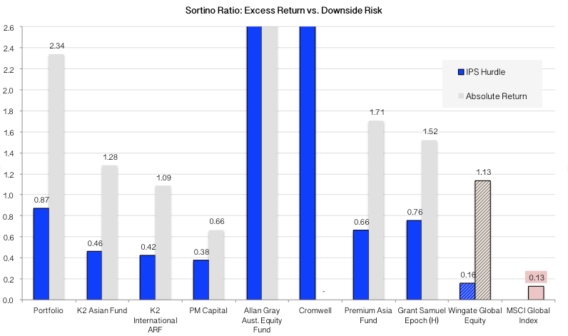
In this analysis Wingate offers a fairly unexciting Sortino Ratio on an IPS-relative basis. The reason for this is that total returns from the Fund have been relatively subdued over recent periods, partly because the manager has taken quite a defensive stance. Because we look at returns relative to IPS, a manager with returns similar to our target will find that their excess return is smaller and returns below the IPS target are more frequent. The Fund’s Sortino on an absolute basis further supports this where it achieves a score of 1.13. Finally we also include the Sortino from the MSCI Global Index. This provides a fairly good benchmark by which to view our portfolio’s results. For example, while we did have a period of very poor returns from PM Capital and our emerging markets funds, we see that on a risk-adjusted basis they actually did quite well. Ideally we want to maintain at a portfolio level an Absolute Return Sortino above 1.0.
Price vs. High Water Mark (HWM)
A High Water Mark is the highest price as asset has achieved over a given time period. The chart below shows the price performance (30 day Moving Average) of the market and Wingate, relative to HWM since July 2012. Studying an asset’s performance relative to High Water Mark helps us understand how deep and long periods of underperformance run. As the chart below shows, Wingate’s performance relative to HWM is much more shallow and stable than the broader market.
A High Water Mark is the highest price as asset has achieved over a given time period. The chart below shows the price performance (30 day Moving Average) of the market and Wingate, relative to HWM since July 2012. Studying an asset’s performance relative to High Water Mark helps us understand how deep and long periods of underperformance run. As the chart below shows, Wingate’s performance relative to HWM is much more shallow and stable than the broader market.
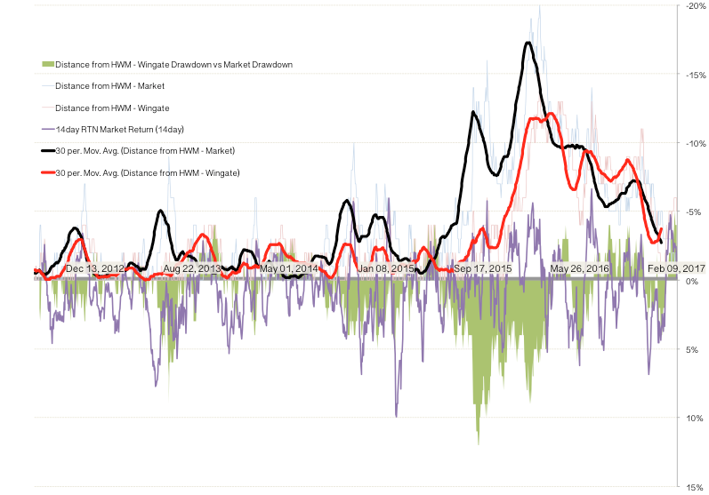
Fund failures and mistakes
We all make mistakes, and Fund managers are no exception. In reviewing the Fund's track record and performance I was most drawn to events of early 2016 where the Fund significantly underperformed, to the extent that it has permanently damaged the Fund's long-term performance statistics. What is important about this is not that they underperformed, but that the underperformance could be explained as an error of judgement and not process. As it turns out, the Fund was caught out by the sharp dive and subsequent recovery between late 2015 and early 2016, failing to use the dip to bolster their equity portfolio exposure. While a mistake in hindsight, their reasons for taking this conservative (and ultimately costly, in a relative sense) position were well-grounded.
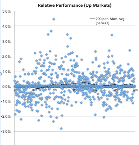
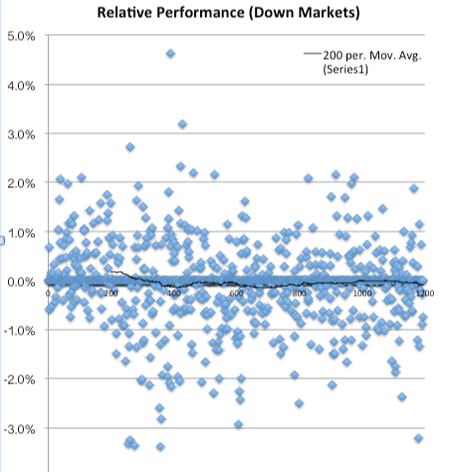
Returns Relative-to-Benchmark
We all make mistakes, and Fund managers are no exception. In reviewing the Fund's track record and performance I was most drawn to events of early 2016 where the Fund significantly underperformed, to the extent that it has permanently damaged the Fund's long-term performance statistics. What is important about this is not that they underperformed, but that the underperformance could be explained as an error of judgement and not process. As it turns out, the Fund was caught out by the sharp dive and subsequent recovery between late 2015 and early 2016, failing to use the dip to bolster their equity portfolio exposure. While a mistake in hindsight, their reasons for taking this conservative (and ultimately costly, in a relative sense) position were well-grounded.
Returns Relative-to-Benchmark
|
|
Summary
We are recommending that <###CLIENT####> invest $280,000 cash into the Wingate Global Equity Fund (Wholesale Units, Unhedged).
As a standalone investment strategy, the Wingate Global Equity Fund targets equity-like returns with substantially less volatility than the broader global equity market. This is achieved through a covered option-writing program that allows the manager to generate additional income while pre-selecting buy and sell points for the manager’s underlying portfolio.
The dynamic nature of this strategy (the crossover point of option strike prices) makes it particularly well suited to portfolios in which investors are more sensitive to sequencing risk, for example retirees and liability-managed strategies.
Similarly, the heavy reliance on option premium income means that the strategy should see an increase in portfolio income during periods of market crisis, reducing the impact of normal market corrections.
Another feature of the strategy is a relatively high level of income and less control over the timing of equity buy and sell points. This means that the potential tax consequences are potentially more severe than traditional equity funds. As a result it provides greatest efficiency within tax-exempt portfolios, or for investors with minimal taxable income.
Finally we have recommended taking a position in the unhedged version of this Fund as we expect the Australian dollar to weaken slightly, to between USD$0.65 and USD$0.71 over the next three years.