A theoretical model for using the TSA Risk-Return Model with Cauchy probability density measure tail risk and options |
October 2017
|
Extending our TSA Breakeven formula, we propose a model that incorporates a modified Cauchy probability density function to better reflect fat-tailed, high-kurtosis returns and reduce dominance of unrealistic forecasts that cluster around historic means. The model is formed by focusing on the incremental changes in probability across the density curve, and scaling our results at Log (p.t / p.t-1). Incorporating this model with our TSA Breakeven formula we also find discrepancies traditional financial models that rely on un-scaled price and volatility estimates, and we suggest one possible use of this formula using an OTM Butterfly strategy.
Part 1: Value at Risk using incremental changes in the probability density function
Our variables are: mean (or FV point estimate), historical volatility and the size of incremental changes in price ("step" size) that we wish to model.
Probability density function is mapped:
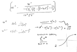
f(x) = 1/(1+(Pi * (x)^2)
We then compare the incremental changes (IC) in probability between each step as:
IC = f(x)t - f(x)t-1 ].
Then incremental changes for each step (ICC):
ICC = IC * Step
We also calculate a scaled version (ICC Converted: ICCC)
ICCC = (IC*Step)/(price at t-1)
Part 2: Scaling VAR in time
Using Y and M to indicate the range of prices we wish to excluded from our analysis (e.g., prices close to the mean; where Y=M all results are included in our analysis) each observation of price, we estimate of the cumulative value as:
VAR+ = Sum ICC from Price Y to infinity
and;
VAR- = Sum ICC from M to zero
These VAR estimates can then be scaled to Y as:
VARLog+ = (VAR+/Y)-1
and;
VARLog- = (VAR-/Y)-1
VAR confidence will be calculated according to the position of Y and M, relative to the current price. If Y=M, results will be VAR 0.50.
Note: A similar operation can be performed on ICCC as: Sum ICCC from Price Y to infinity, and; Sum ICCC from Price Y to zero.
Part 3: "Two Step" level of significance.
We remodel our VARLog for significance in our "Two Step" model^: This transforms the results to show the change (in Log) required to break-even. Where the change is negative, the rate required to recover is larger. This should not replace a model for investor behaviour (prospect theory etc):
TSA.Sig = ABS{([1+VARLog]/1)-1}
For a more complete picture we can combine the results, taking TSA.Sig of VARLog+, and deducting results from those of TSA.Sig of VARLog-. This will bias results to the negative.
^Note: We designed the "Two Step" model as a very simple way of incorporating sequencing risk into our investment models. For example, if prices rise 50% a 33.3*% fall will return us to zero, while a 50% fall will require a 100% return for us to return to breakeven; if the change was 90% instead of 50%, the change second step would now be 47.4% and 1000% respectively. When the range of returns is small these differences are also small, however, as our range of results widen the range of movement required in the next step to return us to breakeven increases exponentially on the upside, while it slows on the downside.
Part 4: Interpreting the results
The combination of results provides a probability distribution that scales for price and adjusts for fat tails. We propose this as a better way than simply bastardising risk estimates by manipulating Kurtosis. Further, our model proves that incremental changes in price leads to exponential increases in per-unit risk. The result provides a distribution bounded by (1/infinity) and infinity. This gives us a better representation of real-life results.
For example, compare the differences in probability (one-tail) under the two models (Normal : New):
*Approximately once every 3.488 million years.
**Approx. once every billion years.
Prospect theory teaches us that it's better to err on the side of caution with these things. Over the last sixty-five years we have only had about 16 times in which the daily return has been equal to or worse than a 6 Standard Deviation event, compared to the 26 predicted by our model. By comparison, a normal gaussian distribution would predict that a 6-Sigma event has about a one in 68,000 chance of having occurred once during this period.
At an individual asset level, values can be more or less bounded than these theoretical models suggest. In the real world a discounted liquidation value may provide a "minimum" amount for which it can be sold. Conversely, if we were using the model to value a zero-coupon Bond where price volatility is estimated at 5%, then a default of the issuer with a 60% return of capital (40% loss) is more likely than a 8-standard deviation event on the upside. This problem is unavoidable. A more accurate way of measuring volatility and risk would be to compare everything to the "liquidation value" of assets, however, even if possible, this is impractical and would change continually as the capital structure and legal obligations of the company changes.
Part 4: Using with TSA Risk-Return Model
The model can be extended with the TSA Risk-Return Model. We will need to consider the conditional probability (as CVAR) for each price not with our estimate of mean and volatility, but also against variables that reflect current conditions. This will produce two sets of data that conflict with each other, except at the point at which current price and volatility aligns perfectly with our fair value estimates (a lazy model of Efficient Markets Hypothesis where markets are both transactionally and price/value efficient).
This makes the calculations more complex. For each observation the "current" scenario will include a price that hasn't been factored into the "historical" estimate, which will widen the two points estimated, relative to what would happen in real life (this may or may not matter, especially if we have a static fair value estimate for our "historical" inputs.
In blending these two point estimates we need to estimate time, so we can model where prices are relative to the cycle. Again this is going to be easier if our fair value or historical mean is stable. Regardless, we can determine time by measuring each price estimate relative to the cumulative probability of the price advancing (if P>mean) or declining (if P<mean). The time estimate we are interested in is from the current price to our target fair value or mean. We err on the side of caution and assume that prices have not reached their extremes yet. Knowing the length of a full cycle we estimate the mid-point (time from mean-to-mean) and then the time from last mean to current price. The remainder is our estimate of time until we return to the mean.
Velocity of prices: In our theory on the velocity of prices (Phase 1 to 3), we suggest that sudden falls in price are more violent than rises, which means that early in a bull market prices may be moving slower than our estimates of time (probability density etc) would suggest. We might need to think of a solution to this...
Time decay: We use time decay to join our two point estimates. If we don't use time decay to join our point estimates the model would tell us any price above the mean plus difference in earnings yield and yield curve is assured of falling. A linear model is also not appropriate as it might lead us to be overconfident in our results. A model with time decay that reflects convexity of time is most appropriate. Here we can estimate the significance of historical data vs current trend data using an exponent of time. For example:
If:
W = time since cycle beginning
O = full cycle term
M = Our level of confidence in cycle term and momentum
exp = exponent of time, a rough estimate is fine, probably 2 or 3
Then:
Weight of Historical point = (O*(1/M))-W)/(W)^(exp)
Blended with our Log model of incremental probability we are provided with a time series for every price, accounting for momentum*. We can also view this as time-series but with return profile for each price point, or with both as a three-dimensional frame.
*Momentum is automatically built into the calculations due to the effect of time decay. As the decline is non-linear and the "current" price, volatility and position in cycle is dependent on price, even if the model predicts we are near the peak of the cycle, the weighting to current data will remain high. This is because as the term outstanding shrinks (the model's way of saying we are near the extreme, and about to experience a retracement), the relative value of time before the cycle ends is increased.
Part 5: Investment ideas
By using a more realistic measure of probability and by scaling our results with respect to price (t-1 Log) and investor behaviour (TSA.Sig) we are better able to identify pricing anomalies. Our model highlights errors in the normal distribution, and the damage caused by underestimating tail risk. In practice we find that traditional pricing models are ill-equipped to handle long tails. Moreover, as price changes and risk are not scaled, volatility models also do not work properly.
Beside helping investors make better informed decisions with regard to portfolio risk management, this model may also have potential as an alternative way of valuing options.
Compare our results to that of the Black-Scholes Model: Our model will suggest that the further Out of the Money (OTM), the more they are mispriced. Further, our model would tell us that Options narrowly in-or-out of the money are overpriced. By extension (and ignoring taxes), investors may find benefit in selling covered Calls close to the money, while buying them significantly OTM.
An even better strategy might be a Butterfly; traditionally this would see an investor buying Calls and Puts ATM, selling twice the quantity OTM, then repurchasing another set even further OTM (so cashflows = $0). We could change the shape of this strategy by moving our strike prices for our starting options slightly OTM, which would allow us to shift the strike prices for all our following options further OTM. At time decay and delta will affect near prices most, a small change in our first set could significantly widen the profit window. Other options might include shortening the "first" profit window by moving our first options OTM but the rest of our first Butterfly intact. The excess cash (which will likely be tiny) can be used to buy options a long way OTM. They will most likely expire worthless (and at the expense of profits between first layer of strikes and third layer of strikes), but if it pays off it could be very profitable. Ie, for a strike equivalent to 3 sigma from the mean, probability of it exercising is very small (0.135%normal), which we would expect to cost ~ 0.25% of the strike. Our model suggests the true likelihood of this event happening is closer to 0.95%. Real life has seen this event happen approx. 0.7% of the time, suggesting a mis-pricing of about 180%.
Our variables are: mean (or FV point estimate), historical volatility and the size of incremental changes in price ("step" size) that we wish to model.
Probability density function is mapped:
f(x) = 1/(1+(Pi * (x)^2)
We then compare the incremental changes (IC) in probability between each step as:
IC = f(x)t - f(x)t-1 ].
Then incremental changes for each step (ICC):
ICC = IC * Step
We also calculate a scaled version (ICC Converted: ICCC)
ICCC = (IC*Step)/(price at t-1)
Part 2: Scaling VAR in time
Using Y and M to indicate the range of prices we wish to excluded from our analysis (e.g., prices close to the mean; where Y=M all results are included in our analysis) each observation of price, we estimate of the cumulative value as:
VAR+ = Sum ICC from Price Y to infinity
and;
VAR- = Sum ICC from M to zero
These VAR estimates can then be scaled to Y as:
VARLog+ = (VAR+/Y)-1
and;
VARLog- = (VAR-/Y)-1
VAR confidence will be calculated according to the position of Y and M, relative to the current price. If Y=M, results will be VAR 0.50.
Note: A similar operation can be performed on ICCC as: Sum ICCC from Price Y to infinity, and; Sum ICCC from Price Y to zero.
Part 3: "Two Step" level of significance.
We remodel our VARLog for significance in our "Two Step" model^: This transforms the results to show the change (in Log) required to break-even. Where the change is negative, the rate required to recover is larger. This should not replace a model for investor behaviour (prospect theory etc):
TSA.Sig = ABS{([1+VARLog]/1)-1}
For a more complete picture we can combine the results, taking TSA.Sig of VARLog+, and deducting results from those of TSA.Sig of VARLog-. This will bias results to the negative.
^Note: We designed the "Two Step" model as a very simple way of incorporating sequencing risk into our investment models. For example, if prices rise 50% a 33.3*% fall will return us to zero, while a 50% fall will require a 100% return for us to return to breakeven; if the change was 90% instead of 50%, the change second step would now be 47.4% and 1000% respectively. When the range of returns is small these differences are also small, however, as our range of results widen the range of movement required in the next step to return us to breakeven increases exponentially on the upside, while it slows on the downside.
Part 4: Interpreting the results
The combination of results provides a probability distribution that scales for price and adjusts for fat tails. We propose this as a better way than simply bastardising risk estimates by manipulating Kurtosis. Further, our model proves that incremental changes in price leads to exponential increases in per-unit risk. The result provides a distribution bounded by (1/infinity) and infinity. This gives us a better representation of real-life results.
For example, compare the differences in probability (one-tail) under the two models (Normal : New):
- 1 Stdev - 16% : 25%
- 2 Stdev - 2.28% : 14.76%
- 3 Stdev - 0.135% : 0.95%
- 4 Stdev - 0.003% : 0.75%
- 5 Stdev - 0.0000287%* :0.61%
- 6 Stdev - 0** : 0.17%
*Approximately once every 3.488 million years.
**Approx. once every billion years.
Prospect theory teaches us that it's better to err on the side of caution with these things. Over the last sixty-five years we have only had about 16 times in which the daily return has been equal to or worse than a 6 Standard Deviation event, compared to the 26 predicted by our model. By comparison, a normal gaussian distribution would predict that a 6-Sigma event has about a one in 68,000 chance of having occurred once during this period.
At an individual asset level, values can be more or less bounded than these theoretical models suggest. In the real world a discounted liquidation value may provide a "minimum" amount for which it can be sold. Conversely, if we were using the model to value a zero-coupon Bond where price volatility is estimated at 5%, then a default of the issuer with a 60% return of capital (40% loss) is more likely than a 8-standard deviation event on the upside. This problem is unavoidable. A more accurate way of measuring volatility and risk would be to compare everything to the "liquidation value" of assets, however, even if possible, this is impractical and would change continually as the capital structure and legal obligations of the company changes.
Part 4: Using with TSA Risk-Return Model
The model can be extended with the TSA Risk-Return Model. We will need to consider the conditional probability (as CVAR) for each price not with our estimate of mean and volatility, but also against variables that reflect current conditions. This will produce two sets of data that conflict with each other, except at the point at which current price and volatility aligns perfectly with our fair value estimates (a lazy model of Efficient Markets Hypothesis where markets are both transactionally and price/value efficient).
This makes the calculations more complex. For each observation the "current" scenario will include a price that hasn't been factored into the "historical" estimate, which will widen the two points estimated, relative to what would happen in real life (this may or may not matter, especially if we have a static fair value estimate for our "historical" inputs.
In blending these two point estimates we need to estimate time, so we can model where prices are relative to the cycle. Again this is going to be easier if our fair value or historical mean is stable. Regardless, we can determine time by measuring each price estimate relative to the cumulative probability of the price advancing (if P>mean) or declining (if P<mean). The time estimate we are interested in is from the current price to our target fair value or mean. We err on the side of caution and assume that prices have not reached their extremes yet. Knowing the length of a full cycle we estimate the mid-point (time from mean-to-mean) and then the time from last mean to current price. The remainder is our estimate of time until we return to the mean.
Velocity of prices: In our theory on the velocity of prices (Phase 1 to 3), we suggest that sudden falls in price are more violent than rises, which means that early in a bull market prices may be moving slower than our estimates of time (probability density etc) would suggest. We might need to think of a solution to this...
Time decay: We use time decay to join our two point estimates. If we don't use time decay to join our point estimates the model would tell us any price above the mean plus difference in earnings yield and yield curve is assured of falling. A linear model is also not appropriate as it might lead us to be overconfident in our results. A model with time decay that reflects convexity of time is most appropriate. Here we can estimate the significance of historical data vs current trend data using an exponent of time. For example:
If:
W = time since cycle beginning
O = full cycle term
M = Our level of confidence in cycle term and momentum
exp = exponent of time, a rough estimate is fine, probably 2 or 3
Then:
Weight of Historical point = (O*(1/M))-W)/(W)^(exp)
Blended with our Log model of incremental probability we are provided with a time series for every price, accounting for momentum*. We can also view this as time-series but with return profile for each price point, or with both as a three-dimensional frame.
*Momentum is automatically built into the calculations due to the effect of time decay. As the decline is non-linear and the "current" price, volatility and position in cycle is dependent on price, even if the model predicts we are near the peak of the cycle, the weighting to current data will remain high. This is because as the term outstanding shrinks (the model's way of saying we are near the extreme, and about to experience a retracement), the relative value of time before the cycle ends is increased.
Part 5: Investment ideas
By using a more realistic measure of probability and by scaling our results with respect to price (t-1 Log) and investor behaviour (TSA.Sig) we are better able to identify pricing anomalies. Our model highlights errors in the normal distribution, and the damage caused by underestimating tail risk. In practice we find that traditional pricing models are ill-equipped to handle long tails. Moreover, as price changes and risk are not scaled, volatility models also do not work properly.
Beside helping investors make better informed decisions with regard to portfolio risk management, this model may also have potential as an alternative way of valuing options.
Compare our results to that of the Black-Scholes Model: Our model will suggest that the further Out of the Money (OTM), the more they are mispriced. Further, our model would tell us that Options narrowly in-or-out of the money are overpriced. By extension (and ignoring taxes), investors may find benefit in selling covered Calls close to the money, while buying them significantly OTM.
An even better strategy might be a Butterfly; traditionally this would see an investor buying Calls and Puts ATM, selling twice the quantity OTM, then repurchasing another set even further OTM (so cashflows = $0). We could change the shape of this strategy by moving our strike prices for our starting options slightly OTM, which would allow us to shift the strike prices for all our following options further OTM. At time decay and delta will affect near prices most, a small change in our first set could significantly widen the profit window. Other options might include shortening the "first" profit window by moving our first options OTM but the rest of our first Butterfly intact. The excess cash (which will likely be tiny) can be used to buy options a long way OTM. They will most likely expire worthless (and at the expense of profits between first layer of strikes and third layer of strikes), but if it pays off it could be very profitable. Ie, for a strike equivalent to 3 sigma from the mean, probability of it exercising is very small (0.135%normal), which we would expect to cost ~ 0.25% of the strike. Our model suggests the true likelihood of this event happening is closer to 0.95%. Real life has seen this event happen approx. 0.7% of the time, suggesting a mis-pricing of about 180%.
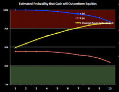
Probability Density Estimates for TSA Breakeven
|
TSA Breakeven Sample Output
|
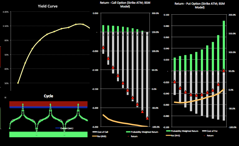
TSA Breakeven model showing Cycle Measurement and BSM Pricing
|