Data analysis tools & spreadsheets
The following is a small selection of the spreadsheets, dashboards and applications I have built and use within my business.
|
Managing Portfolio Risk over the long term


|
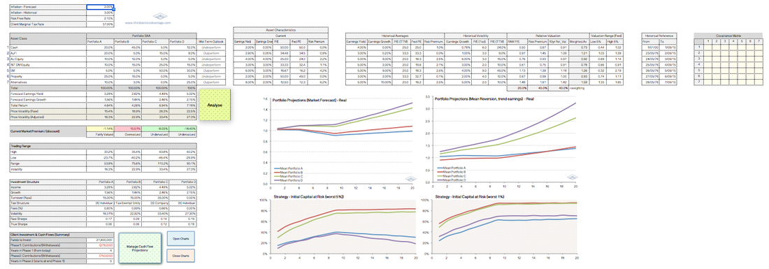
One of the greatest challenges any investment advisor must face is building investment portfolios when market and asset analysis provide widely conflicting views as to an asset's prospects, and suitability for the client.
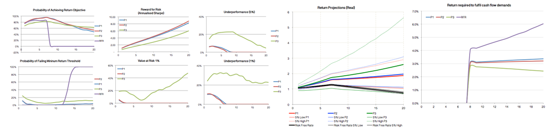
Using a current example, while one set of data may suggest US equities are moderately overvalued, another may argue that the price is justified due to a low interest rate environment or strong near-term earnings growth. This simulator attempts to illustrate both the problems and opportunities this can create. Broken down to it's most basic level, if we can agree that over the very long term an investor's return (expressed as CAGR) should reflect the rate of real (inflation-adjusted) earnings growth, less tax and fees, then we also be able to agree that most volatility is due to investors (subjective) pricing of those earnings[1]. If this assumption is right, then over the very long term (multiple decades) investor return forecasts should be calculated on long-term real earnings growth and volatility on the value of their investment re-based / adjusted to reflect current market anomalies (i.e., where asset prices are under/over valued). Of course undertaking this type of analysis will inevitably cause inaccurate short-term forecasts, but over the long term it can offer valuable insights by estimating the return from assets on both a historical (investment capital adjusted) basis, as well as based on shorter-term market forecasts. This enables us to determine whether an asset that may currently look very expensive is, in fact, a better investment proposition than an asset that looks very cheap but still offers a lousy return. This simulator uses three measures of relative value (forward P/E, Risk Premium and 10-Year compound return) with the user able to adjust the settings to suit their own opinion of relevance. Of course we could complete this analysis using some fairly basic maths, but it would be challenging to make sense of how this might interact with an investor's cash flows. This simulator simplifies this process and allows the user to manipulate data to ensure a more thorough analysis of portfolio outcomes. This spreadsheet runs a series of Monte Carlo simulations, separating the four portfolios into eight different accounts, each of which run 10,000 independent trials over 20 time periods while incorporating the client's cash flow requirements/contributions (to correct for sequencing risk). Volatility and returns are modelled on an after-tax basis. Although time periods are, by default, illustrated in single-year increments this can be easily adjusted by changing return and volatility inputs (ie., to adjust to period (n) from annualised return/volatility statistics: returns = r^(n), volatility = vol*(sqrt(n)) ). [1] This forms a topic for a considerable amount of research and literature that suggests an inverse relationship between the level of dividends paid and asset volatility. An extension of this is the seemingly conflicting finding that franking credits are not fully valued by the market. One possible explanation for this is anchoring and mental accounting. I have also included our general formula for measuring downside risk. I developed this as a way to quickly and cleanly quantify downside risk under various scenarios. Here, we measure the cumulative cash flows of a risky asset against a low-risk asset on a comparable investment horizon. Therefore we use the yield curve as our yardstick, not the cash rate. This gives us the potential alpha for the risky asset (or portfolio). To this we add 1, then divide the current market price of the asset (or market's) earnings: this gives us an approximate of the level at which earnings must be priced for the risky asset to deliver the same return as the low-risk asset. Once we have this we can compare this against a range of factors, such as current price of earnings, historical price of earnings, or target price of earnings (the list is nearly limitless). We do this by measuring the quantum of change required, divided by the volatility of the factor, multiplied by the period of our analysis. |
|
Schiller CAPE Analysis (R, Shiny)
|
An interactive dashboard illustrating the distribution of the Cyclically Adjusted Price-Earnings Ratio (Case-Shiller PE, or CAPE).
This application was built using R (code), with graphics interface loaded through Shiny App. Data sourced from Professor Shiller (Yale University), with CSV files uploaded from Quandl. Current to July 2017. |
|
4Sight

|
4Sight is a trading simulator designed to help advisers test, learn from, and improve their investment decision-making processes.
Unlike traditional portfolio and risk simulators which "normalise" the statistical properties and behaviour of assets, 4Sight uses an algorithm that takes real-world (non-parametric) returns and incorporates exogenous economic, political, environmental and market events. Importantly, while the data driving the simulator is real, to encourage investors to look at the data supporting their investment decisions, the names of countries have been changed. Also unlike most simulators, investment costs are included, as are alternative assets such as residential real estate and commodities. To test the investor's skill level, 4Sight also pits the investor against other investors, each of which is programmed to implement their own unique investment style. Background The ideas behind 4Sight not only come from observing the behaviour of investors (and investment advisers) but also from the growing body of research into neurofinance which finds that investors' decision-making process and abilities are often influenced by the body's physiological responses to stimuli (in particular the cognitive response to fluctuations in testosterone and cortisol). Learning to compensate for, if not control, one's biases (emotional, cognitive and chemical) sets the framework for a more rational, robust and consistent approach to investment and risk management. In Development: 4Sight+ 4Sight+ will allow the user to run their portfolio (in the simulation environment) as a professional investment fund. This includes modeling fund flows based on both relative and absolute performance (after-fees), as well as business and staff costs. The idea to include these features comes from the observation that many investors are willing to underperform, and pay higher fees, so long as returns were not negative, while many investors feel compelled to withdraw from financial investments or managers if their performance is negative, even returns were better than their peers. |


|
Monte Carlo Simulation - Portfolio modelling
|
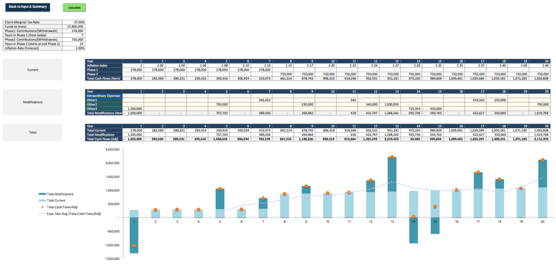
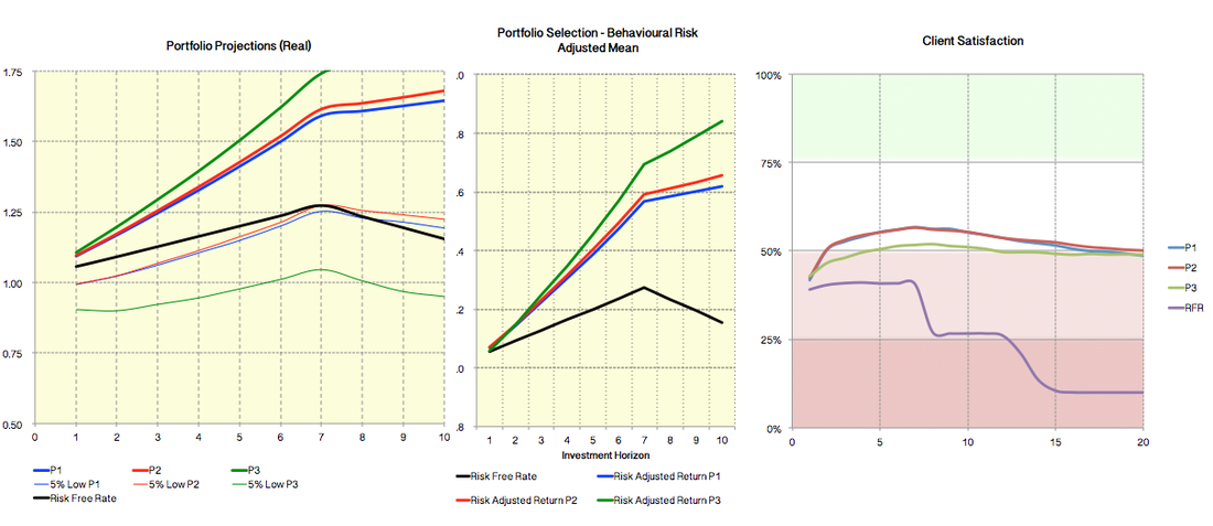
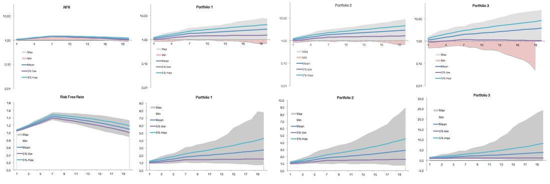
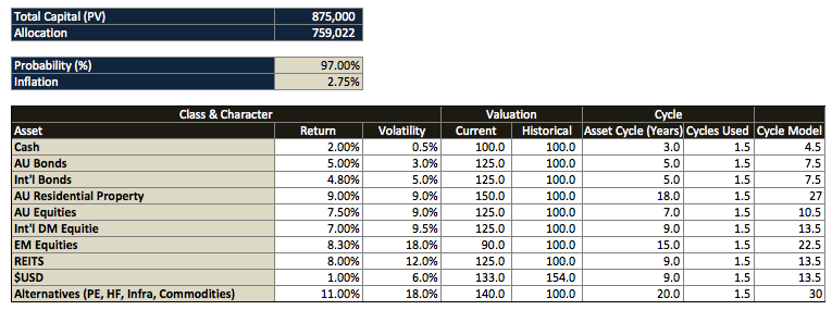
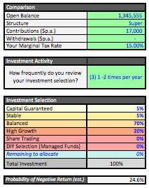
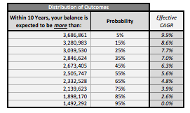
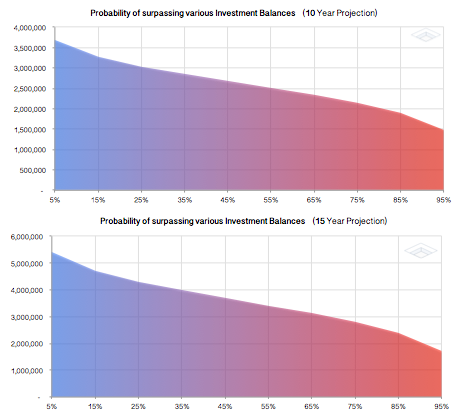
This Monte Carlo simulator provides a comparison of three portfolios (plus Risk Free Rate), with ability to incorporate the impact of tax, fees, composition of returns, portfolio turnover, return objectives and inflation.
Importantly the simulation allows us to take into account the client's cash flows (contributions/withdrawals). This allows the user to consider how a static portfolio (i.e, constant Strategic Asset Allocation) might be expected to perform. Analysis includes the following:
Incorporated in the analysis are several qualitative factors, such as the client's personality and the importance of reaching certain goals. This includes two questions to assess the client's attitude toward statistically measurable risks that tend to elicit emotional rather than rational responses (gambling question and insurance question). In this simulator we try to capture client reactions to potential loss both as probability of loss, and magnitude of loss. Based on evidence presented by Kahneman, Tversky and others, we see that people tend to make decisions that are overly reliant on mental accounting biases. This means that even if we know how a client feels about a specific level of risk for one specific event, we cannot extrapolate this to describe how they would react to another event For example, if a person is presented with a gamble where heads they win $100 and tails they win nothing, and they tell us they would be willing to pay $35 for such a bet, then we might expect them to pay $70 for the same gamble but with $200 prize money. In reality they tend to become more cautious as the stakes risk. However, if the gamble was framed in reverse, and the outcomes offered potential losses, then we might expect the investor to become more risk-seeking. This illustrates the non-linear nature of risk and loss aversion. In the spreadsheet this flows through to two charts: "Portfolio Selection - Behavioural Risk Adjusted Mean", and "Client Satisfaction". Note: As it stands today, I do not use these qualitative aspects to determine a client's portfolio. Rather this was an exercise in thinking about how client questionnaires and risk profiles may be better administered to clients (this is perhaps a job for a psychometrician to develop further?).
| ||
|
Portfolio Optimisation (non Markowitz)
|
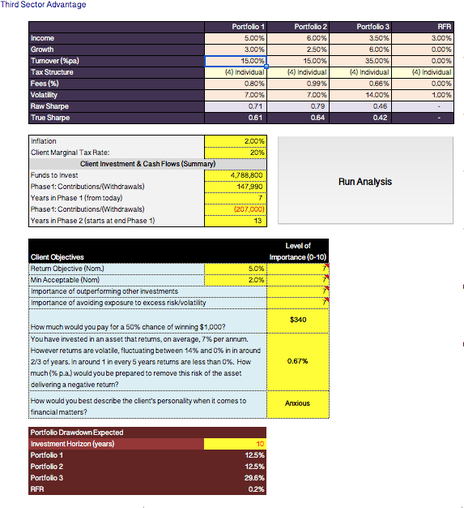
This is a simpler, arguably more user-friendly version of the portfolio optimisation tool above.
Here we are trying to determine our optimal asset allocation by comparing the risk and return trajectory of each individual asset, and using these results to inform match a portfolio for each future cash flow (adjusted by the client with a cash flow projection table), at a stated level of confidence. In essence, the matching of cash flows to assets is comparable to Asset Liability Matching. The difference between this and a basic volatility-adjusted return matrix is that we are also trying to account for pricing disparity and consumer risk preferences. We need a number of steps to achieve this:
|
|
Managing Downside Risk
|
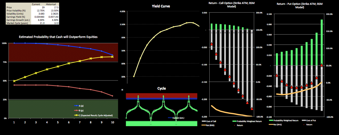
"Assets look expensive, but we're not in a bubble"
This is something I hear fairly often, and while I don't disagree, I believe it can also lull investors into a false sense of security. Just because long-term returns may be our primary focus, does not mean we should remain idle. Rather we need to rephrase the debate. The question should not be "are we at the peak", but rather "over the next X-years, am I likely to be compensated for risk". Here risk includes all forms of market risk: risk of permanent loss of capital, illiquidity, volatility etc etc.. Our model attempts to provide some colour around the likelihood of event occurring in which the investor will be financially worse off if they invest (or retain) a risky asset versus a risk-less alternative. Our model Here we use an extension of our general formula for measuring downside risk (see formula in slide), but take it a step further by estimating the probability of mean reversion given an asset's position in a normal cycle. To explain why this is important, let's say we had an asset had a long-term fair value of $100, with a standard deviation of $25, but was trading at $150, then the probability of mean reversion multiplied by the relative impact[1] of this reversion over the very short term would be greater than if we were measuring the probability over a longer timeframe. In essence, the formula produces a result that is more confident over short periods and less confident over longer periods. However, as we are not attempting to guess the returns for the coming week or even the coming year (to believe we can would be foolish), we must adjust our calculations to reflect current market sentiment and the natural ebbs and flows of markets. Therefore in this model we attempt to identify where we are in the cycle. From here we measure the distance from today to mean reversion, then apply a function to estimate the trajectory between current prices and the long-run mean (which, for the purpose of this model we assume is approximately 'fair value'). From these estimates we can estimate the probability that a risky asset will underperform a risk-free benchmark (being zero-coupon bond at year n). The final element in this model is an estimate of returns from ATM options (both Calls and Puts) at the model price forecast; this enables the user to easily see the return profile of each set of options, but more importantly allows us to estimate the cost of "insurance". For example, if we have a significant tax liability that we wish to carry to future years, if may make more sense to retain our asset and buy Put options, or simply sell Call options over our existing position. In these types of scenarios the relative "cost" may be much lower than if we simply sold the assets. [1]This is because, in the case of investment assets, risk premiums are factored in; thus while "riskier" assets will generally have greater volatility in price, for this volatility the investor is compensated (volatility, size, liquidity etc). |
|
Property vs Shares (Simulator)
|
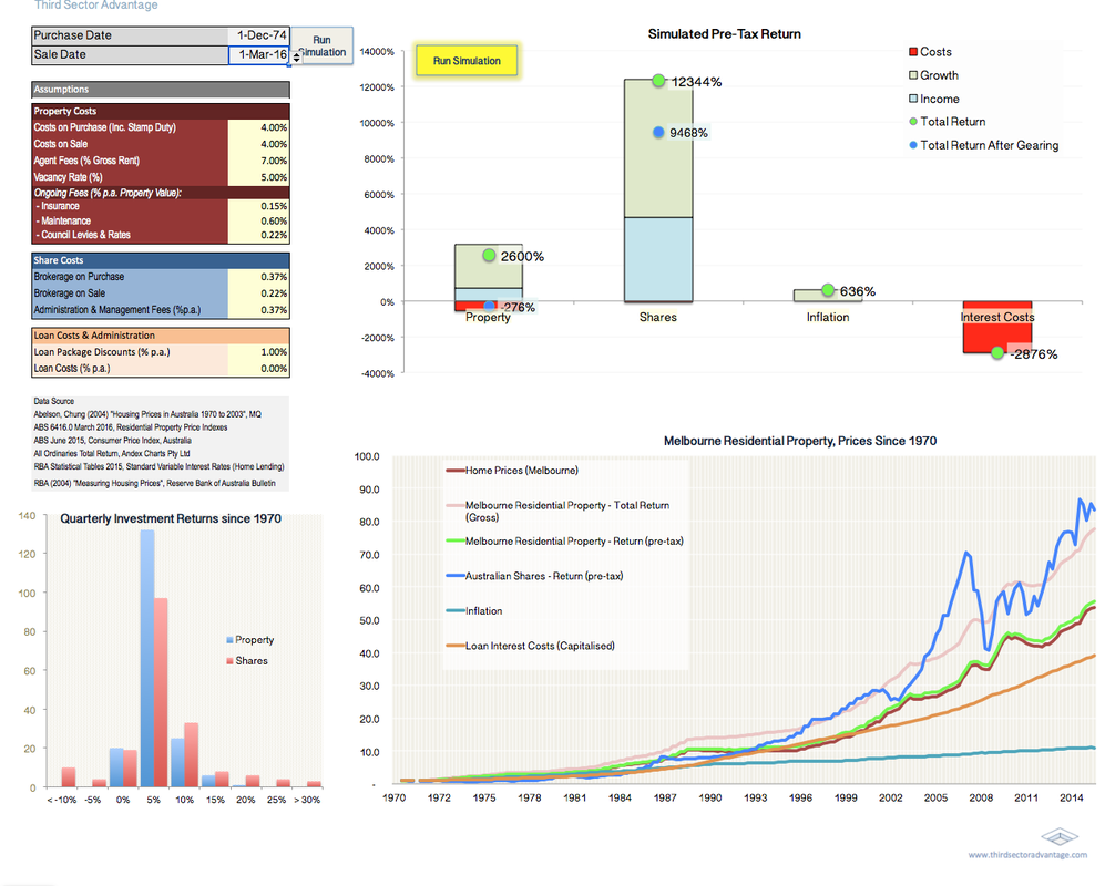
Despite roughly 40% of Australians' private wealth being tied up in residential property (predominantly the family home) most investors and advisers hold a somewhat distorted, over-romantisiced view of property as an investment class.
Of course this is not entirely unexpected. Not only because of the tendency for investors to treat anecdotal and empirical evidence as equals but because the other key source of information tends to be from real estate agents, "advertorials" and industry associations. The objective of this simulator is to not only help clients gain a better understanding of property, but also to help other advisers illustrate to their clients the inherent risks and costs associated with property investment. |
|
Superannuation Fund Review (2017)

|
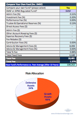
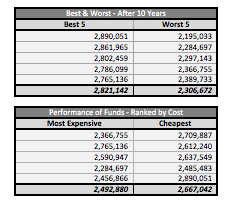
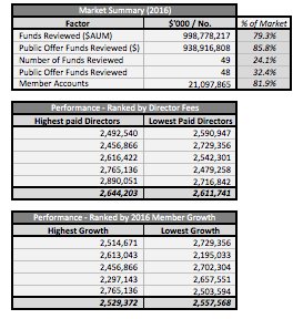
For many people, choosing a superannuation fund can be a daunting task. This calculator was prepared to help simplify the process.
Here we compare Australia's largest 49 public offer funds which together represent over 21 million individual accounts, with a total value of approximately $1 trillion, or 79% of the total assets managed by APRA regulated funds. In addition to analysing fund performance and fees, our analysis considers client cash flow (contributions and withdrawals), investment strategy, taxation, and member engagement in order to identify the funds most likely to meet their requirements. |

|
Retirement, Savings & Quality of Life
|
I built this calculator to help illustrate to clients the effect that small changes to savings and expenses can have on their retirement, and in particular the "first phase" of retirement, which we describe as being the time between ones retirement and the point at which they become less active (normally from about 80 years of age).
We find it important to discuss this with our clients as focusing only on their finances may lead many to work longer than they want, and in doing so quickly erode the time they have to pursue their retirement goals such as travel, active family time and involvement in their local communities. For example, in the example to the right, this person's goal of retiring at 62 years of age is achievable, and from their current age and position results in about 37% of their future life being spent saving (working), 35% in active retirement (Phase 1), and 28% in the second phase of their retirement. If, however, they reduced their household expenses by about 6% they could change these proportions to 22, 50% and 28% (a 40% increase in their active retirement years). |
|
Life Expectancy Calculator
|
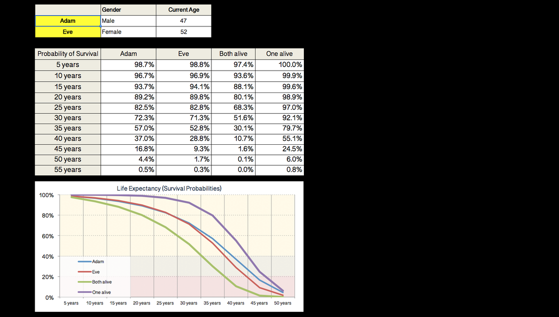
Based on Australian Life Tables (2014), this simple life expectancy calculator is designed to help with client discussions around issues such as capital adequacy and the risks of outliving their retirement savings.
|
|
Volatility-adjusted returns: adjusting for time, cash flows and leverage


|
The question "is volatility risk?" is a bit like asking whether the sky is blue: the answer reflects an individuals interpretation of the question.
Over the past decade designing portfolios for, and consulting with, investors large and small, the volatility/risk debate is still the one I find most intriguing. Part of this, I believe, is because for most of us the idea of losing money makes us feel very uncomfortable, even if it's only a temporary "paper loss". The idea of redeeming your money today for less than you may have had a day, week or month earlier, strikes fear into many investors' hearts. This fear is even more powerful when an investor seems helpless to take action to recover those losses (such as contributing more to their savings). With emotions running high, it's not surprising we see many investors continue to make irrational decisions; for example, people who, on the day of their retirement move all their wealth to cash, despite the thirty or more years of retirement ahead of them. For some, the prospect of a slow and steady errosion of their wealth is better than the somewhat bumpier flight path offered by a diversified portfolio. Of course, if we were being truly rational, each individual investor's focus should be on maximising the value of their wealth at a predetermined and specific point in the future. Risk in this case can be viewed in probabilistic terms: what are the chances I will not reach this goal? What is the probability of landing at each point above or below this goal? Etc.,etc.... In some ways it is fortunate that most people don't think this way. Not only would this put many investment advisers out of a job, but it would likely result in problems raising capital and would make tools such as monetary policy much less effective. Nevertheless, if we, as individual investors, take the effort to differentiate between volatility and risk, considerable benefits await. Long-term investors with a tolerance for risk can be paid for their ability to stay the course. Liquidity premiums, additional risk premia (in particular through non-market-cap sector allocation), generally more favourable tax treatment, and the sensible use of leverage. This spreadsheet seeks to provide a simple illustration of how an investor should allocate their capital over their stated investment horizon while factoring in their comfort level with debt. To do this each portfolio is modelled independently with their returns over time discounted to volatility in order to reflect (with the stated confidence level) the minimum level of return the portfolio would be expected to achieve. This incorporates the client's cash flows. By laying each of these "risk adjusted" portfolios side-by-side we can determine which one provides the best risk-adjusted return. This is assumed to be the most appropriate asset for the client to select. Also illustrated are the expected return and portfolio value if the client's "exit" date were pushed back 10 years or brought forward 10 years. Importantly, "exit" date is just meant to infer an arbitrary "investment horizon" used by clients. For example, let's say the aforementioned recent retiree is 65 years of age and uncomfortable investing beyond 5 years, even though he is in good health and expected to live into his nineties. By educating our clients and quantifying the difference in prospective return and potential risk we find many investors become much more accepting of volatility and comfortable taking a long-term view of their investment journey. |
|
Income Tax Calculator

|
A quick and easy Income Tax calculator (based on tax rates announced in the 2016 Federal Budget).
|