What can past returns tell us about future risk and returns?
Experiment writing trading and back-testing algorithms in Python (020218)
Background
In this experiment, I set out to test the relationship between recent performance, time, and liquidity. The strength of these relationships should provide an indication as to whether mean-reversion or momentum strategies are dominant over the market cycle.
In this experiment, I set out to test the relationship between recent performance, time, and liquidity. The strength of these relationships should provide an indication as to whether mean-reversion or momentum strategies are dominant over the market cycle.
Process
To test the relationship between these investment styles, we first separated the market into high trade volume and low trade volume. Within each of these categories, qualifying stocks were ranked by decile on their performance from the last 5, 10, 15, 20 and 30 days; from each of these data points we then measured the forward week return. Data was recorded and rebalanced on a weekly basis. Our sample period covered the ten years from 1 February 2008 to 31 January 2018. Data categories and filters include:
To get around this (and to experiment with Quantopian's backtesting IDE) I wrote an algorithm in Python to do most of the heavy lifting for us.
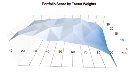
Our first step is to sort the data to convert the problem from two three-dimensional layers (time and liquidity) into a series of two-dimensional portfolios. We do this by sorting the data by liquidity (2 categories) and performance decile (10 categories), and then by Lookback Period (5 categories). This produces 100 two-dimensional portfolios from which we can compute our basic portfolio statistics (Alpha, Beta, Sharpe, return and drawdown). It also makes it much less computationally intensive, reducing the data load per trial to about 2.08 million data points. At this point we are only interested in gathering results from a long-only portfolio (because of the ranking system, the results would look something like a momentum strategy for well-performing stock, and a mean-reversion strategy for the worst performing stock).
The next step was to write code to handle the performance of the remaining portfolio. I wrote an algorithm that called the security prices (US Equity market; c. 4,000 stocks) before using Quantopian's Pipeline function to filter and group: first by trade volume, then by performance decile. I then ordered the algorithm to make an equal-weight investment in each qualifying stock at the start of the week (Monday), before liquidating the entire portfolio before trade the following Monday, then doing it all over again (in the real world this would be very messy, however as we are ignoring taxes and brokerage costs it's the simplest way of extracting the information that we need). We used the S&P500 as our benchmark.
At the end of the analysis period, the summary results were transferred to an Excel spreadsheet where I loaded a simple macro to compare the results and identify "Qualifying Portfolios" based on client objectives (i.e., preference for high sharpe) and rules (i.e., at least 1% Alpha and Beta 0.2 below mean).
To test the relationship between these investment styles, we first separated the market into high trade volume and low trade volume. Within each of these categories, qualifying stocks were ranked by decile on their performance from the last 5, 10, 15, 20 and 30 days; from each of these data points we then measured the forward week return. Data was recorded and rebalanced on a weekly basis. Our sample period covered the ten years from 1 February 2008 to 31 January 2018. Data categories and filters include:
- Liquidity categories x 2
- Performance Decile x 10
- Lookback periods x 5
- Rank Record (p.a.) x 52
- Years Backtest x 10
To get around this (and to experiment with Quantopian's backtesting IDE) I wrote an algorithm in Python to do most of the heavy lifting for us.
Our first step is to sort the data to convert the problem from two three-dimensional layers (time and liquidity) into a series of two-dimensional portfolios. We do this by sorting the data by liquidity (2 categories) and performance decile (10 categories), and then by Lookback Period (5 categories). This produces 100 two-dimensional portfolios from which we can compute our basic portfolio statistics (Alpha, Beta, Sharpe, return and drawdown). It also makes it much less computationally intensive, reducing the data load per trial to about 2.08 million data points. At this point we are only interested in gathering results from a long-only portfolio (because of the ranking system, the results would look something like a momentum strategy for well-performing stock, and a mean-reversion strategy for the worst performing stock).
The next step was to write code to handle the performance of the remaining portfolio. I wrote an algorithm that called the security prices (US Equity market; c. 4,000 stocks) before using Quantopian's Pipeline function to filter and group: first by trade volume, then by performance decile. I then ordered the algorithm to make an equal-weight investment in each qualifying stock at the start of the week (Monday), before liquidating the entire portfolio before trade the following Monday, then doing it all over again (in the real world this would be very messy, however as we are ignoring taxes and brokerage costs it's the simplest way of extracting the information that we need). We used the S&P500 as our benchmark.
At the end of the analysis period, the summary results were transferred to an Excel spreadsheet where I loaded a simple macro to compare the results and identify "Qualifying Portfolios" based on client objectives (i.e., preference for high sharpe) and rules (i.e., at least 1% Alpha and Beta 0.2 below mean).
Results (Liquid Portfolios)
We start by looking at the results from our liquid portfolios. We find that mean reversion is by far the dominant factor in liquid portfolios, though it is more reliable in predicting future under-performance than out-performance. Moreover, those that have suffered the worst recent returns (worst 5%) are likely to continue under-performing. In fact, we found the highest Sharpe Ratios occurred in the 2nd and 3rd deciles (when ranking low to high). In contrast, the very best performers (best 1%) sustained the heaviest draw-down, worst return and lowest Sharpe.
We start by looking at the results from our liquid portfolios. We find that mean reversion is by far the dominant factor in liquid portfolios, though it is more reliable in predicting future under-performance than out-performance. Moreover, those that have suffered the worst recent returns (worst 5%) are likely to continue under-performing. In fact, we found the highest Sharpe Ratios occurred in the 2nd and 3rd deciles (when ranking low to high). In contrast, the very best performers (best 1%) sustained the heaviest draw-down, worst return and lowest Sharpe.
|
|
Are the results useful?
We have to be careful not to read too much into the results, especially as we are modelling a relatively short period (10 years) which includes the Global Financial Crisis and subsequent recovery. That aside, the bottom 50% of the market (decile 1:5) all significantly outperformed the top 50% of the market over all look-back periods, with only the worst 1% recording significant underperformance.
We have to be careful not to read too much into the results, especially as we are modelling a relatively short period (10 years) which includes the Global Financial Crisis and subsequent recovery. That aside, the bottom 50% of the market (decile 1:5) all significantly outperformed the top 50% of the market over all look-back periods, with only the worst 1% recording significant underperformance.
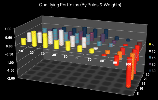 Example of Qualifying Portfolios: Factors: 3.5*SR -0.3*Beta + 1*Alpha; Rules: High liquidity + Sharpe>-1mu + Beta<+1mu + Alpha>-1mu
On the surface, this would suggest there is an opportunity for traders to enhance portfolio returns and/or reduce risk by concentrating their exposure on the most liquid but worst-performing stock.
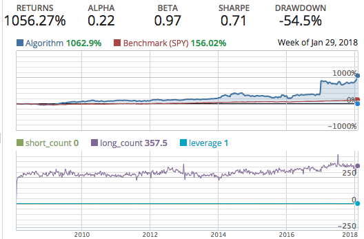
By way of example, had we taken a levered equal-weighted exposure (150%) to the worst performing 30% of the market (ex very-worst 5%), while taking a short position (-100%) in the best performing 20% of the market, we would have seen the following changes to our investment results:
By way of example, had we taken a levered equal-weighted exposure (150%) to the worst performing 30% of the market (ex very-worst 5%), while taking a short position (-100%) in the best performing 20% of the market, we would have seen the following changes to our investment results:
- Return: +4.6% p.a.
- Beta: -0.34
- Sharpe Ratio: +0.18
- Max Drawdown: -16.72%
Results (Illiquid Portfolios)
Next we turn to the results from our illiquid portfolios (lowest 25% of market by trading value). Here the results become much more interesting .
As we would expect results were much more pronounced, with higher highs and lower lows across all measures, however, we also saw evidence of the best performing illiquid stocks continuing to outperform by a significant margin, seemingly supporting a momentum-based approach.
Summary
These conflicting results are extremely interesting. Could it be that both mean-reversion and momentum styles work, but at different stages of a stock size or maturity?
If so, this might suggest that we can use this information to help "weed out" stocks from our trading algorithm; for example, take long positions in the best performing illiquid and worst performing liquid, and take short positions in best performing liquid stocks (short position in worst performing illiquid might not be feasible, particularly when slippage is taken into consideration).
More research is needed, however, this provides a starting point to evaluating the relationship between past and future performance.
Note: It would be very computationally intensive, but theoretically it should be possible to setup a neural network (Machine Learning) to measure and compare the performance of all these factors over time. This would be particularly helpful from a risk management perspective, as it could tip of the investor (or algorithm) as to a change (strengthening, weakening or reversal) in the pattern
Example of a simple portfolio: Liquidity category: 25%-50% Recent Performance: worst 10%
|
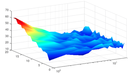
We can also use the data to model three-dimensional planes through MATLAB
|
Model attributes:
Algorithm was built in Python and deployed via Quantopian using data from Quandl. 100 independent trials covering 2,000 stocks (4,000 / 2 liquidity filters) across 520 rebalancing periods. Approximately 208 million data points. Supplementary analysis (factor and rules based weightings) conducted through Excel.
Reference material:
Algorithmic Trading: Winning Strategies and Their Rationale, Chan, Ernest
Liquidity as an Investment Style, Ibbotson, R., Chen, Z, et al (https://www.cfapubs.org/doi/sum/10.2469/faj.v69.n3.4)
Kalman Filtering and Neural Networks, Haykin, Simon
GNU Octace (www.gnu.org)www.quantconnect.com
www.quantiacs.com
www.quantopian.com
www.quandl.com